Real space renormalization of the self-avoiding walk
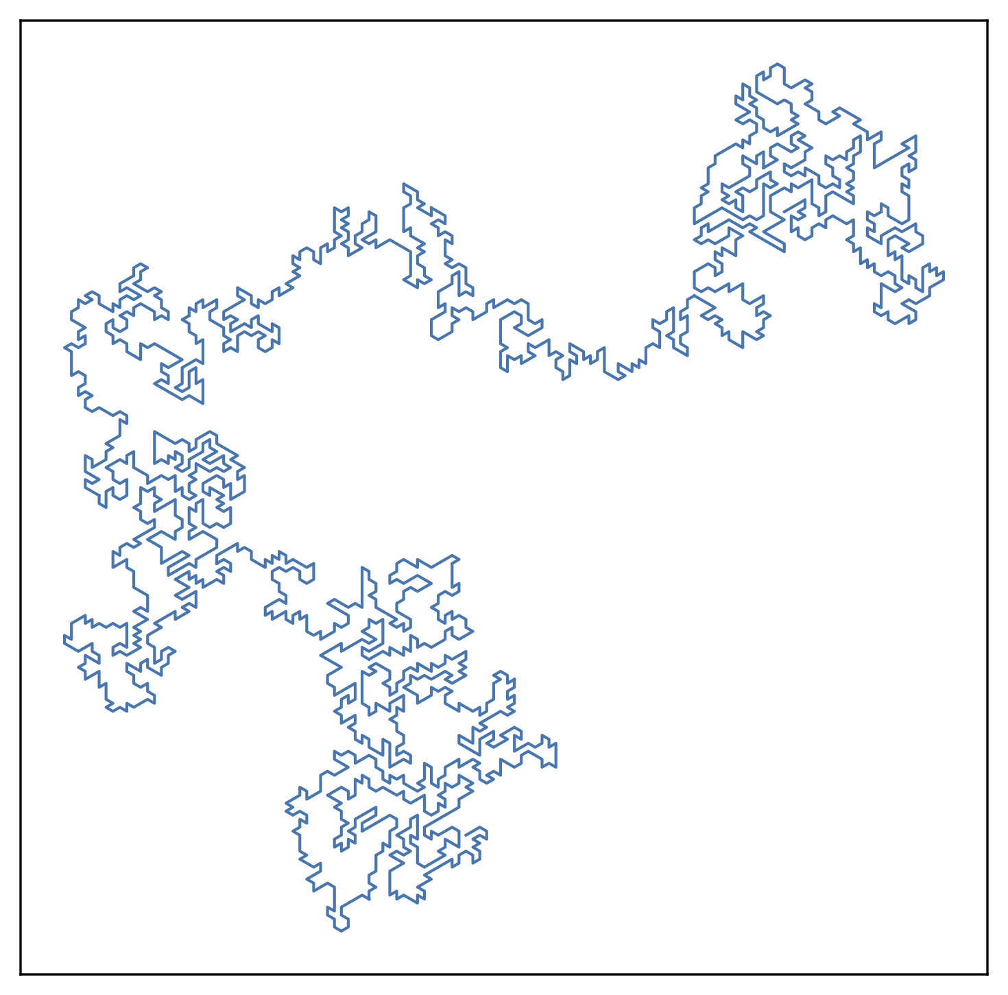
Random walks are stochastic processes where the position of a walker at a given time \(T\) is the sum of a number \(N\) of random variables with \(N\) scaling as \(T\). These random walkers are permitted to visit the same location multiple times. Here we will consider a model of a self avoiding walk which is similar to a random walk in some ways, but crucially different in others. The physical motivation comes from long string-like objects: polymers are a good example, DNA being perhaps the most famous. The essential question we will try to answer is how the distance between the ends of a polymer chain of length \(L\) scales with \(L\), averaged over all configurations of the polymer chain which do not involve self-crossings. See here for some more notes on the self-avoiding walk, and a discussion of how this problem is related to critical phenomena in models of magnets. In this post we will explore a different (and more transparent) route to understanding the self avoiding walk, and will in fact be able to estimate the scaling of the linear size of the polymer chain with \(L\) by means of a renormalization group argument similar to the one discussed for percolation here.
One of the arguments we will discuss is from the book Introduction to Renormalization Group Methods in Physics by Creswick, Farach and Poole. Variants of the argument appeared in work by Shapiro and Napiorkowski et al in the late 1970s: we will also briefly discuss this more involved kind of approximation.
The self-avoiding walk
As discussed above, the self avoiding walk is a statistical mechanical model of a polymer chain. Allowed configurations of a chain composed of \(n\) links are any configurations which do not contain self-intersections. There are many more configurations in which the chain is crumpled than straight: these therefore might hint that the end-to-end distance of the chain (in Euclidean space) scales sublinearly with \(n\): we will say that \(|\vec R| \sim n^\nu\) for some power \(\nu<1\). It is known that if the chain were allowed to have self intersections, then it would just trace out a random walk, and we would have \(\nu=1/2\). The question is what the effect of self avoidance is, and how it depends on the spatial dimension in which the chain is embedded.

The generating function
In order to understand the behavior of the self avoiding walk, it will be useful to consider the partition function of the walk. Let us say that the beginning of the chain is at the origin, and the end is located at some position \(\vec R\). Since all configurations which do not self-intersect have the same probability in the ensemble we are considering, and therefore the same energy, we can write the partition for a length-\(n\) chain as
\[M_n = \sum_{\vec R} M_n(\vec R)\]where \(M_n(\vec R)\) is the number of self avoiding walks of \(n\) links which connect the origin to \(\vec R\). They key step that will allow us to frame the self avoiding walk as a critical phenomenon and extract its properties using renormalization group methods is the introduction of a grand canonical partition function in which we sum \(M_n\) over \(n\), with appropriate weighting that depends on \(n\) via the exponential of a chemical potential that one can think of as a fugacity. In other words, we allow the number of links in the self avoiding walk to vary, and introduce a parameter \(K\), which is like \(e^{\mu/T}\) for temperature \(T\) and chemical potential \(\mu\), which controls the number of links in the chains that dominate the sum over \(n\). Defining this grand canonical partition function
\[G(K) = \sum_{n} K^n M_n\]will be important for the steps that follow.
The critical point
In particular, the behavior of the partition function as we vary \(K\) will display a nonanalyticity which will allow us to interpret the exponent \(\nu\), which describes the dependence of the extent of the chain on its length, as a critical exponent that can be estimated by an approximate renormalization group scheme. An important assumption is that \(M_n\), the total number of self-avoiding walks of \(n\) steps starting from the origin, scales with \(n\) as
\[M_n \sim K_c ^{-n} n^{\gamma-1}\]for some constant \(K_c>1\). This captures the exponential dependence on \(n\) along with power law piece with exponent \(\gamma\). Here we can see that in the sum for \(G(K)\) there is a competition between the exponentials \(K^n\) and \(K_c^{-n}\). As we vary the fugacity \(K\), there will be a transition in our partition function when \(K\) crosses through \(K_c\). With our form for \(M_n\), we can write our partition function as
\[Z(K) = \sum_n \left(\frac{K}{K_c}\right)^n n^{\gamma-1} = \sum_n e^{-\kappa n} n^{\gamma-1},\]where we have defined \(\kappa = -\log(K/K_c) \approx 1 - \frac{K}{K_c}\) for \(K\) just below \(K_c\). (This is analogous to a reduced temperature that is often defined in critical phenomena: it vanishes at the critical point.)
Therefore we can see (by converting \(Z(K)\) into an integral over \(n\) and making a change of variables to \(\kappa n\)) that \(Z(K)\) diverges as \(\kappa^{-\gamma}\) as \(\kappa\) is lowered to zero. We can also see that the dominant \(n\) in the sum for \(Z(K)\) diverges as \(\kappa^{-1}\): this can be seen from a saddle point approximation of
\[Z(K) \approx \int_0^\infty e^{-\kappa n} n^{\gamma-1}.\]Therefore, if we are interested a correlation length, defined as
\[\xi^2(K) = \frac{\sum_{\vec R}\sum_n |\vec R|^2 K^n M_n(\vec R)}{Z(K)},\]then it will diverge as \(\xi(K)\sim \kappa^{-\nu}\), given the fact that \(\lvert\vec R\rvert\sim n^\nu\).
Having set up the self-avoiding walk as a critical phenomenon with the fugacity as the control parameter, we are now in a position to estimate the exponent \(\nu\) through constructing an approximate real space renormalization group.
Renormalization group transformation
The goal is to successively coarse-grain our self-avoiding walk by zooming out to larger and larger scales, lumping the small-scale features into effective features on larger scales. As we zoom out to longer lengthscales, we will account for the loss of resolution of small-scale processes by renormalizing the fugacity: therefore the value of \(K\) will be lengthscale dependent. Because of the emergent scale-invariance at the critical point, we expect a fixed point in the map relating the fugacity at small lengthscales to that at large lengthscales. However this fixed point is unstable: moving the initial value of \(K\) away from the fixed point causes the RG to map us either to zero or infinite fugacity, as we will see below.
It is important to note that there are a number of different approximations that should yield qualitatively the same results, but which will provide different estimates for quantities such as the critical exponent \(\nu\). We will discuss two such approximations below, and work out the simplest case. In the simplest one, there is only one parameter that flows with lengthscale: the fugacity \(K\). Once and also try to do better by accounting for effective types of steps in the self-avoiding walk that are generated by coarse-graining but are not present at the smallest scale: this necessitates the introduction of other parameters whose flows must be tracked: we do not discuss in depth.
Simplest case
This RG scheme is discussed in the book by Creswick et al mentioned above. The basic idea is to consider zooming out on our system by a factor of two at a time. This will require collapsing e.g. a \(32\times 32\) grid into a \(16\times 16\) grid, and then into a \(8\times 8\) grid, and so on. Recall the the value of the fugacity defines a statistical weight assigned to each self avoiding walk starting at the origin: this weight depends only on the length of the walk. As we coarse-grain the system, there will be many walks on a small scale that get coarse-grained into the same large scale walk: therefore it is necessary to renormalize our fugacity so that the weight assigned to a walk at half of our current resolution (i.e. after one step of coarse graining) is the sum of the weights of all the walks that would be coarse-grained to this result. Note that we also would like a coarse-graining procedure that preserves the self-avoiding property of the walk, since this is expected to be crucial to its long lengthscale behavior, and allows to capture the behavior on large scales by the same model that we use on small scales, with different effective parameters.

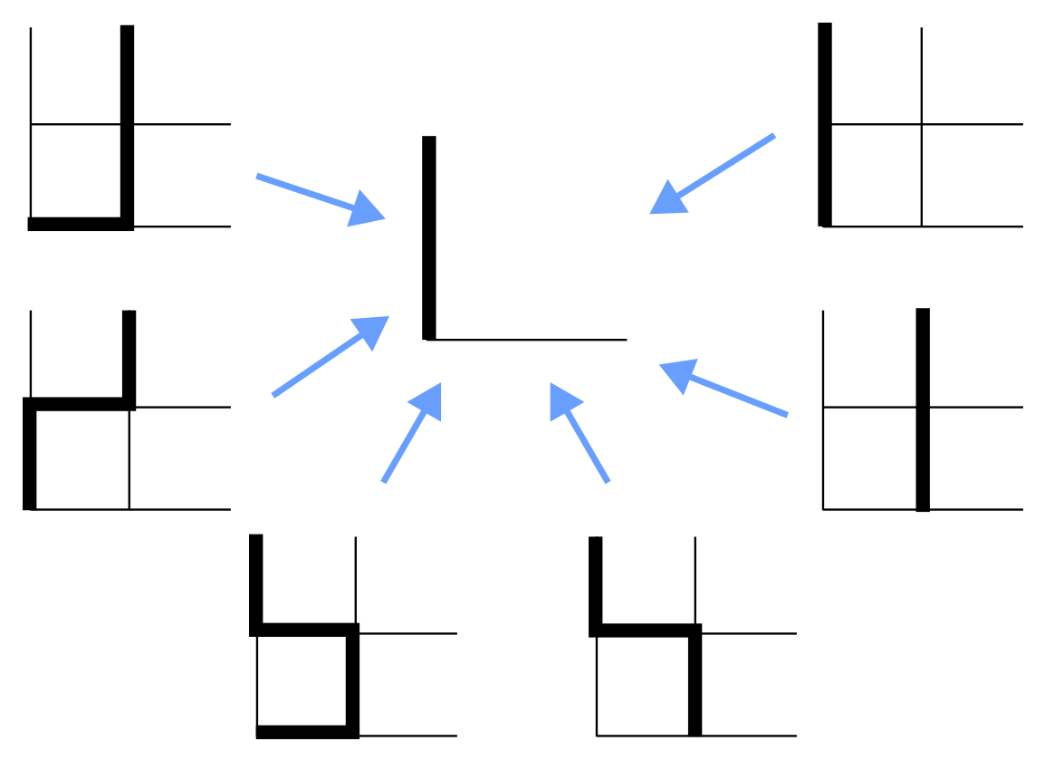
Some choices are required to make this process well-defined. In particular, since we are allowing ourselves to renormalize only one parameter, the fugacity, we will have to make some omissions in the types of steps that our coarse-graining captures. Below we show the coarse graining scheme, which maps paths on a \(2\times2\) grid to a path on the \(1\times1\) grid. We consider only paths that go from bottom to top of the cell: other directions can be dealt with in the same way due to the symmetry of the lattice. Note also that we coarse-grain non-overlapping sections of the lattice: this is why the unit being coarse grained contains a bottom edge and left edge but no top or right side edge.

The omissions come from the renormalization scheme we have chosen: in essence this can be thought of as restricting the set of self-avoiding walks under consideration, which is an approximation we make for the sake of consistency of our RG scheme. Given the diagram oulined above, we can write down an equation for the renormalized fugacity when we cut our resolution in half. There are 2 paths composed of 3 links, two paths composed of 2 links, and one path composed of 4 links that get renormalized to a single upward step. Therefore the renormalized fugacity, denoted \(K'\), in terms of the original fugacity \(K\), is
\[K' = K^4 + 3 K^3 +2 K^2.\]As we iterate this map, we obtain the effective fugacity governing the self-avoiding walk on larger and larger scales.

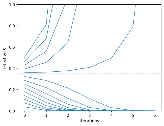
As seen in the figure above, the RG transformation has stable fixed points at 0 and \(\infty\) and an unstable fixed point at \(K = K^*\approx 0.32\), above which an initial condition flows to \(K\to\infty\) and below which an initial condition flows to \(K\to0\). The unstable fixed point is the critical point, and the behavior of the RG map around this fixed point allows to estimate the exponent \(\nu\), which governs the correlation length. In particular, we can ask how many RG steps are needed for an almost-critical system with fugacity \(K^*+\delta\) to look clearly in one phase or the other. Close to the critical point we can linearize our recursion relation to obtain, for small \(\delta\),
\[\delta' = 2.38\times \delta,\]which tells us that close to criticality the correlation length, defined as \(2^q\) where \(q\) is the number of RG steps needed for \(\delta\) to become \(O(1)\), diverges as
\[\xi \sim \delta^{-1/\log_2(2.38)}\approx \delta^{-.80}.\]Therefore our RG scheme yields a correlation length exponent \(\nu\) of \(0.80\). It turns out that in two dimensions, \(\nu\) for the self-avoiding walk is known exactly (through different methods) to be \(0.75\), which is in the ballpark of our rough RG-based estimate. We could also extend our approximate RG to three or higher dimensions, though this would require some combinatorics to count paths of various lengths from one side of the coarse-grained cell to another.
Extensions
In the previous scheme we allowed ourselves only to renormalize a single parameter: the fugacity. Therefore we had to make some arbitrary choices for our coarse-graining, focusing on walks which could be split up into the \(2\times 2\) chunks drawn above, and ignoring more complicated configurations which don’t neatly fit into this single-fucagity framework.
An apparently more thorough approach is to consider the fact that our renormalization can generate “interactions” which are not present in the bare model but which we need to keep track of as we go to larger and larger lengthscales. This is a generic property of renormalization group transformations: most useful RG transformations somehow truncate the types of interactions generated under coarse-graining so that one can focus on an interpretable part of coarse-grained system, as we did in previously keeping all the information in a single parameter: the renormalized fugacity. It is possible to allow another type of interaction (a different type of step, for example a coarse-graining of a \(2\times2\) grid with links forming a pattern not included in the set of six shown above) to be generated by the RG, and concurrently track the flows of two fugacities rather than one. One can in principle extend this to an arbitrary number of fugacities for different types of steps on the lattice which are generated by coarse-graining, limited only by patience.
We will not discuss this implementation in detail here, but it is done so in two different ways in works of Shapiro and Napiorkowski et al, as referenced in the Introduction.