Percolation and renormalization group
Thanks to Ariel Amir for introducing me to this argument, now published in his book Thinking Probabilistically.
Consider a percolation model in 2D (for concreteness, we will envision site percolation, though it turns out that bond percolation has the same critical behavior). In other words, we have an \(L\times L\) square lattice where each vertex of the lattice is either colored in or not, independently with probability \(p\). We are interested in the probability that there exists a path hopping only across colored lattice sites that connects the left side of the lattice to the opposite right side. Clearly when \(p=1\) we will always be able to hop from one side to the other, and when \(p=0\) this will never be possible. A remarkable fact (and the object of our study) is that the probability of being able to percolate from one side of the lattice to the other goes from \(0\) to \(1\) sharply at some critical value of \(p\) between \(0\) and \(1\), in the limit that \(L\to\infty\).
In other words, for large lattices, there is a sharp transition between percolating with probability \(0\) and probability \(1\), which occurs (for site percolation — the model we have described here) at a critical \(p\) of approximately \(p_c\approx 0.59\), as found by numerics. Our goal here will be to provide some intuition as to why this behavior occurs, as well as show how to use a heuristic coarse-graining procedure to obtain properties of the system close to its critical point.
[A side note: we have been talking about a critical point without specifying an order parameter. If this bothers you, the order parameter that one can think of is the probability that a randomly chosen point in the lattice is part of the largest connected cluster of colored sites — this cluster becomes infinite above the transition and so this probability becomes nonzero. This probability vanishes for \(p<p_c\) and becomes nonzero continuously for \(p>p_c\), with its dependence on \(p-p_c\) defining a magnetization exponent \(\beta\)]
Since we are interested in the \(L\to\infty\) limit, it will be useful to thinking about coarse-graining a particular realization of the site coloring to ask about long-lengthscale properties of the lattice: in particular, whether it admits a percolation path from one side to the other. Consider the following coarse-graining plan:
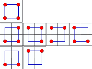
Consider a square lattice of size \(2^n\times 2^n\). We can then impose a hierarchical division of this lattice into blocks, with each block being split into \(4\) blocks of the next-lowest size, arrayed in a \(2\times2\) fashion. This will continue all the way down until each block is a single site on the lattice. We will now find a way to relate the percolation probability at one scale to the scale directly above this one. Start with the smallest scale. The probability of each site being colored is \(p\). Then the probability of a \(2\times2\) block of these sites percolating from left to right is the sum of the probabilities of the different ways in which this can happen. Certainly if \(3\) or more of the sites are colored, then the \(2\times 2\) block percolates. If \(2\) of the sites are colored, then we need these to be in line from left to right, which can happen in two different ways. Therefore the probability of the \(2\times 2\) block percolating is
\[p' = f(p) = p^4 + 4 p^3(1-p) + 2p^2 (1-p)^2.\]Therefore we have devised an approximate relation between the probability of a percolation at a particular scale and at a twice-zoomed out scale. Now if we want the probability of a \(4\times 4\) block of sites percolating, we can reapply this logic, since the block of \(4\) is nothing but a \(2\times2\) block of \(2\times 2\) blocks. Note that our relation between the percolation probabilities at different scales is an approximation because it is possible for a bigger block to percolate without the individual subblocks percolating in the manner that we have prescribed. However, let us be courageous and see where this approximation takes us.
Now that we have a map between percolation probabilities from one scale to another, we can iterate this map to find the percolation probability of an infinite lattice — this probability will correspond to a fixed point of the map \(f(f(\cdots f(p)))\). One can see by inspection that \(p=1\) and \(p=0\) are fixed points of the map, i.e. \(f(p)=p\). These are stable fixed points of the map, in the sense that if \(p\) is perturbed slightly away from them —though between \(0\) and \(1\) — it will return to these fixed points. What are the other two fixed points? We can solve the polynomial equation \(f(p)=p\) to find that they are \(\frac{1}{2}(\pm\sqrt 5 -1)\). One of these is negative — and therefore inaccessible starting from an initial \(p\) which is between \(0\) and \(1\). The other is \(p_c= \frac{1}{2} (\sqrt 5-1)\approx 0.62\). This is an unstable fixed point of the map, in sense that starting at \(p=p_c+\delta p\) and iterating the map will take one to \(1\) or \(0\) depending on whether \(\delta p\) is positive or negative. Note that this critical probability of \(0.62\) is remarkably close to the value of \(0.59\) found much more carefully for numerics on huge system sizes. The fact that it is larger than \(0.59\) reflects the fact that we have left out certain ways to percolate from the left to the right (those which don’t percolate through the subblocks) and therefore need a higher \(p\) to achieve percolation in this truncated definition than in the full model.
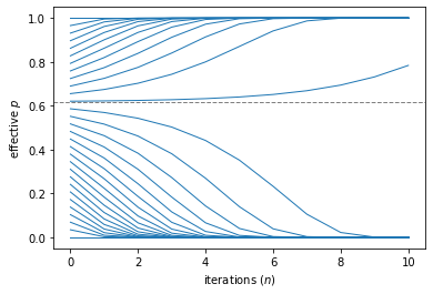
We are now equipped to understand qualitatively the phase diagram of percolation, through an approximate coarse-graining process. We see that for \(p<0.62\), zooming out makes the probability of percolating smaller, and for \(p>0.62\) the probability of percolating increases. Right at the critical point of our coarse-graining map, the system looks self-similar and the percolation probability is independent of length scale, but on either side of this critical point, the system “flows” to either an effective \(p=0\) fixed point, below the transition, or a \(p=1\) fixed point above the transition. The character of the flows right around the critical point — which is an unstable fixed point of the coarse-graining map — can allow us to estimate a critical exponent, which we will now do.
The critical exponent that we will look at is \(\nu\), the correlation length exponent. The correlation length, denoted \(\xi\), is expected to diverge in the vicinity of a second order transition as \(\xi \sim |p-p_c|^{-\nu}\), where the exponent \(\nu\) (unlike, e.g. the critical probability \(p_c\)) is a universal quantity that depends only on the spatial dimension of the lattice, and does not depend on the lattice type or the particular percolation model (bond, site. etc). What does the correlation length mean for percolation? \(\xi\) tells us what the characteristic length scale of the system. One way to think about it is as the linear extent of the largest finite cluster of colored sites in the lattice. This is finite below the percolation threshold, and diverges as an infinite cluster emerges at the transition. It is then finite above the transition again, as there is a single infinite cluster and all other clusters are finite. Therefore if one looks at the probability that two sites separated by distance \(r\) are both in the largest connected cluster, this probability decays at big \(r\) as \(e^{-r/\xi} + f^2\), where \(f\) is the fraction of sites occupied by the biggest connected cluster. Another way to think about \(\xi\) (which may be more relevant in this context) is as the length scale over which one must view the system before the system looks definitively in one phase or the other (percolating or non-percolating). Since the clusters in the system are of typical size \(\xi\), one must zoom out to a lengthscale \(\xi\) in order to truly assess which phase the system is in.
With this in mind, how can we estimate \(\nu\) from our renormalization-group map \(f(p)\)? Imagine we start off-criticality, i.e. \(p = p_c +\delta p\) where \(p_c = \frac{1}{2}(\sqrt{5}-1)\). Then, after one application of \(f(p)\), we have (via a linearization of our map for small \(\delta p\))
\[f(p_c+\delta p) -p_c \approx 2 p_c^2 - p_c^4 -p_c - 4(p_c^3-p_c)\delta p = 2(3-\sqrt 5)\delta p.\]In other words, the effective distance from criticality has growth by a factor of \(2(3-\sqrt 5)\), upon rescaling length by a factor of \(2\). Note that \(2(3-\sqrt 5)>1\), as we know should be the case since \(p_c\) is an unstable fixed point of the map, so perturbations grow under iteration. As we continue to iterate the map, the effective distance from the critical point, quantified by the size of \(\delta p\), will grow exponentially. In fact, defining \(\lambda = \log_2[2(3-\sqrt 5)]\), we can write
\[\delta p \sim 2^{\lambda n}\delta p_0,\]where \(n\) is the number of coarse-graining steps, and \(\delta p_0\) is the initial distance from criticality. The system stops looking critical once \(\delta p\) is \(O(1)\) — in this case the coarse-grained system looks far enough from criticality that is is easy to tell whether it is in the non-percolating or percolating phase. Given the exponential growth of \(\delta p\) under repeated coarse-graining, we can see that the number of steps in order to reach \(\delta p\sim O(1)\) is
\[n \sim \frac{1}{\lambda}\log_2 (1/\delta p_0).\]The length scale by which we coarse grain in order for the system to look non-critical is therefore
\[\xi \sim 2^n \sim \delta p_0^{-1/\lambda}.\]Here we have identified the correlation length with this coarse-graining length scale needed in order for the system to look firmly in one phase or the other — or equivalently — for \(\delta p\) to look \(O(1)\). Therefore we have an estimate of \(\nu = 1/\lambda \approx 1.64\). The exact result for \(2\) dimensions is \(\nu = 4/3\), so we are reasonably close.
In summary, we have seen how a simple renormalization-group argument has led us to decent estimates of the critical point and correlation length exponent for 2D percolation, and perhaps more crucially, a qualitative understanding of coarse-graining in terms of flows of the system under rescaling. Note also that the arguments here can easily be generalized to higher dimensions and different lattice geometries!